Hessian-based uncertainty quantification
Author: James R. Maddison
This notebook describes the use of tlm_adjoint for Hessian-based uncertainty quantification. The approach is based on the method described in
Tobin Isaac, Noemi Petra, Georg Stadler, and Omar Ghattas, ‘Scalable and efficient algorithms for the propagation of uncertainty from data through inference to prediction for large-scale problems, with application to flow of the Antarctic ice sheet’, Journal of Computational Physics, 296, pp. 348–368, 2015, doi: 10.1016/j.jcp.2015.04.047
We assume real spaces and a real build of Firedrake throughout.
Uncertainty quantification problem
We consider the advection-diffusion equation in the unit square domain
for some real and positive \(\kappa\) and subject to doubly periodic boundary conditions. We consider a continuous Galerkin finite element discretization in space and an implicit midpoint rule discretization in time, seeking \(u_{n + 1} \in V\) such that
with timestep size \(\Delta t\) and given some suitable discrete initial condition \(u_0 \in V\). Here \(V\) is a real continuous \(P_1\) finite element space whose elements satisfy the doubly periodic boundary conditions, and after discretizing we have \(m \in V\). For a given value of \(m\) we let \(\hat{u}_N ( m )\) denote the solution obtained after \(N\) timesteps. Given an observation for \(\hat{u}_N ( t )\), \(u_{obs} \in V\), we seek to infer information about the control \(m\). Here we are specifically seeking to infer the transport, defined in terms of a stream function \(m\), which transports the solution from \(u_0\) to \(u_{obs}\) in time \(T\).
We first need to model the observational error. For a given value of the control \(m\) we treat observations are being realizations of a Gaussian random variable, with mean given by \(\hat{u}_N ( m )\), and with known covariance. Specifically we define a density \(p ( u_{obs} | m )\) whose negative logarithm is (up to a normalization term which is neglected here)
\(R_{obs}^{-1}\) is a bilinear and symmetric positive definite observational inverse covariance operator. Here we choose \(R_{obs}^{-1}\) by defining
where \(\mathcal{L}_{\sigma,d} : V \rightarrow V\) is defined by
In the continuous and \(\Omega = \mathbb{R}^2\) case \(R_{obs}\) then defines a covariance operator with single point variance \(\sigma_R^2\) and autocorrelation length scale \(d_R\) (see Lindgren et al 2011, doi: 10.1111/j.1467-9868.2011.00777.x).
We next introduce a prior for the control. We consider a Gaussian prior with mean zero and with known covariance. Specifically we define a prior density \(p ( m )\) whose negative logarithm is (again up to a normalization term)
\(B^{-1}\) is a bilinear and symmetric positive definite observational inverse covariance operator. Here we choose \(B^{-1}\) by defining
Now applying Bayes theorem we obtain a posterior density whose negative logarithm is (up to a normalization term)
We have made a number of modelling choices, but subject to these choices the posterior density now completely describes the information we have about the control after being supplied with an observation \(u_{obs}\). The challenge is that the posterior is defined in a high dimensional space, and is in general not Gaussian. To simplify the problem we approximate the posterior with a Gaussian, and specifically make the approximation (up to a normalization term)
The mean of the Gaussian approximation is set equal to the posterior density maximizer (the Maximum A Posteriori estimate), \(m_{map}\). The inverse covariance of the Gaussian approximation, \(\Gamma_{post}^{-1}\), is set equal to the Hessian, \(H\), of the negative log posterior density \(-\ln p ( m | u_{obs} )\), defined by differentiating twice with respect to \(m\) and evaluated at the posterior density maximizer.
Unfortunately in order to quantify uncertainty we require information about the covariance, and not the inverse covariance. Specifically if we have a linear observational operator \(q \in V^*\) then our estimate for the variance associated with \(q ( m )\) is
which requires access to information about the Hessian inverse.
In the following we use two approaches to gain access to this information.
A low rank update approximation. We approximate the Hessian inverse using a low rank update to the prior covariance, using the methodology of Isaac et al 2015, doi: 10.1016/j.jcp.2015.04.047.
By computing the Hessian inverse action using a Krylov method, preconditioned using the low rank update approximation.
To solve this problem we need several pieces:
A differentiable solver for the forward problem. We will construct this using Firedrake with tlm_adjoint.
To find the posterior maximizer. We will use gradient-based optimization using TAO.
To find a low rank update approximation for the Hessian inverse. We will find this using a partial eigenspectrum obtained using SLEPc.
To compute the Hessian inverse action. We will compute this using a Krylov method using PETSc, preconditioned using the partial eigenspectrum.
Forward problem
We first implement the forward model using Firedrake with tlm_adjoint.
[1]:
%matplotlib inline

from firedrake import *
from tlm_adjoint.firedrake import *
from firedrake.pyplot import tricontourf

import matplotlib.pyplot as plt
import numpy as np

reset_manager()
clear_caches()

mesh = PeriodicUnitSquareMesh(40, 40, diagonal="crossed")
X = SpatialCoordinate(mesh)
space = FunctionSpace(mesh, "Lagrange", 1)
test = TestFunction(space)
trial = TrialFunction(space)

T = 0.5
N = 10
kappa = Constant(1.0e-3, static=True)
dt = Constant(T / N, static=True)
sigma_R = Constant(0.03)
d_R = Constant(0.1)
sigma_B = Constant(0.025)
d_B = Constant(0.2)
u_0 = Function(space, name="u_0").interpolate(
    exp(-((X[0] - 0.4) ** 2 + (X[1] - 0.5) ** 2) / (2 * 0.08 * 0.08)))
u_obs = Function(space, name="u_obs").interpolate(
    exp(-((X[0] - 0.6) ** 2 + (X[1] - 0.5) ** 2) / (2 * 0.08 * 0.08)))


def L(sigma, d, q):
    u = Function(space)
    solve(inner(trial, test) * dx
          == (1.0 / sqrt(4.0 * np.pi * sigma * sigma))
          * ((1.0 / d) * inner(q, test) * dx + d * inner(grad(q), grad(test)) * dx),
          u, solver_parameters={"ksp_type": "preonly",
                                "pc_type": "cholesky"})
    return u


def L_inv(sigma, d, q):
    u = Function(space)
    solve((1.0 / sqrt(4.0 * np.pi * sigma * sigma))
          * ((1.0 / d) * inner(trial, test) * dx + d * inner(grad(trial), grad(test)) * dx)
          == inner(q, test) * dx,
          u, solver_parameters={"ksp_type": "preonly",
                                "pc_type": "cholesky"})
    return u


def R_inv_term(q):
    L_q = L(sigma_R, d_R, q)
    LL_q = L(sigma_R, d_R, L_q)
    return Functional(name="J_mismatch").assign(0.5 * inner(LL_q, q) * dx)


def R_inv_action(q):
    L_q = L(sigma_R, d_R, q)
    LL_q = L(sigma_R, d_R, L_q)
    return assemble(inner(LL_q, test) * dx)


def B_inv_term(q):
    L_q = L(sigma_B, d_B, q)
    LL_q = L(sigma_B, d_B, L_q)
    return Functional(name="J_prior").assign(0.5 * inner(LL_q, q) * dx)


def B_inv_action(q):
    L_q = L(sigma_B, d_B, q)
    LL_q = L(sigma_B, d_B, L_q)
    return assemble(inner(LL_q, test) * dx)


def B_action(q):
    u = Function(space)
    solve(inner(trial, test) * dx == q,
          u, solver_parameters={"ksp_type": "preonly",
                                "pc_type": "cholesky"})
    Li_q = L_inv(sigma_B, d_B, u)
    LiLi_q = L_inv(sigma_B, d_B, Li_q)
    return LiLi_q


def forward(m):
    m = Function(space, cache=True).assign(m)
    u_np1 = Function(space, name="u_np1")
    u_n = u_0.copy(deepcopy=True)
    eq = EquationSolver(inner(trial, test) * dx
                        + 0.5 * dt * inner(dot(perp(grad(m)), grad(trial)), test) * dx
                        + 0.5 * kappa * dt * inner(grad(trial), grad(test)) * dx
                        == inner(u_n, test) * dx
                        - 0.5 * dt * inner(dot(perp(grad(m)), grad(u_n)), test) * dx
                        - 0.5 * kappa * dt * inner(grad(u_n), grad(test)) * dx,
                        u_np1, solver_parameters={"ksp_type": "preonly",
                                                  "pc_type": "lu"})
    for _ in range(N):
        eq.solve()
        u_n.assign(u_np1)

    u_mismatch = Function(space, name="u_mismatch").assign(u_n - u_obs)
    J_mismatch = R_inv_term(u_mismatch)
    J_prior = B_inv_term(m)
    return J_mismatch, J_prior, J_mismatch + J_prior, u_np1
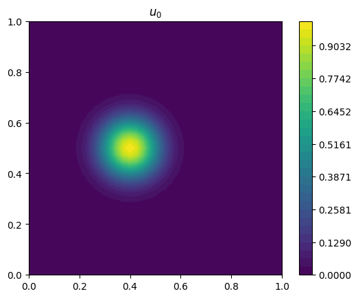
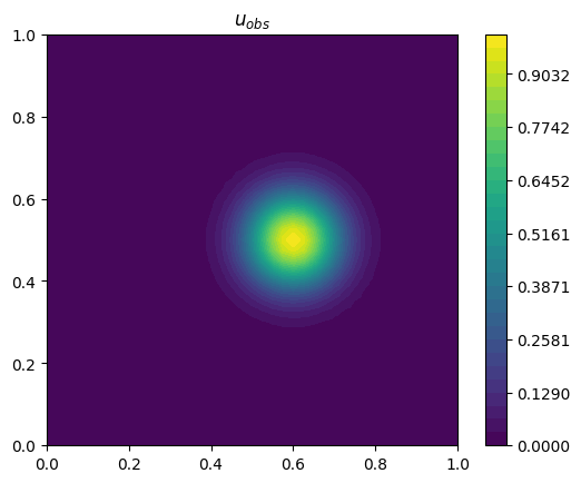
Let’s first visualize the initial condition \(u_0\) and the observation \(u_{obs}\) taken a time \(T\) later.
[2]:
def plot_output(u, title):
    r = (u.dat.data_ro.min(), u.dat.data_ro.max())
    eps = (r[1] - r[0]) * 1.0e-12
    p = tricontourf(u, np.linspace(r[0] - eps, r[1] + eps, 32))
    plt.gca().set_title(title)
    plt.colorbar(p)
    plt.gca().set_aspect(1.0)


plot_output(u_0, r"$u_0$")
plot_output(u_obs, r"$u_{obs}$")
Quantities of interest
In the following discussion we seek to quantify uncertainties in quantities of interest. These are defined using linear functionals, say \(q \in V^*\). Given some value of the control \(m\), \(q ( m )\) is the value of the quantity of interest. Moreover, given the Maximum A Posteriori estimate \(m_{map}\) for the control (the posterior density maximizer), the estimate for the posterior mean of the quantity of interest is given by
To obtain uncertainty estimates we need a covariance operator. Note that a covariance operator, say \(\Gamma_{post}\), is a bilinear operator, \(\Gamma_{post} : V^* \times V^* \rightarrow \mathbb{R}\). It takes the linear functionals we use to obtain values for two quantities of interest, and gives us a value for a covariance between them. In particular the estimate for the posterior uncertainty in a single quantity of interest, defined by a linear functional \(q \in V^*\), is
Finding the posterior maximizer
We now find the posterior density maximizer, which corresponds to seeking a minimum of the negative log posterior density. We solve this problem using the Toolkit for Advanced Optimization (TAO), with the Limited-Memory Variable Metric (LMVM) approach. This is a gradient-based approach, so let’s first verify the adjoint using Taylor verification.
[3]:
m_0 = Function(space, name="m_0").interpolate(
    0.06 * sin(2 * pi * X[1]))

reset_manager()
start_manager()
_, _, J, _ = forward(m_0)
stop_manager()

dJ = compute_gradient(J, m_0)
dm = Function(space, name="dm").interpolate(
    sin(4 * pi * X[0]) * cos(6 * pi * X[1]))
min_order = taylor_test(lambda m: forward(m)[2], m_0, J_val=J.value, dJ=dJ, dM=dm, seed=1.0e-6)
assert min_order > 1.99
Error norms, no adjoint   = [1.53027865e-04 7.39407643e-05 3.63270898e-05 1.80027218e-05
 8.96115500e-06]
Orders,      no adjoint   = [1.04935252 1.02532416 1.01283075 1.00645844]
Error norms, with adjoint = [1.02926724e-05 2.57316785e-06 6.43291602e-07 1.60822709e-07
 4.02054503e-08]
Orders,      with adjoint = [2.00000013 2.00000081 2.00000172 2.00000815]
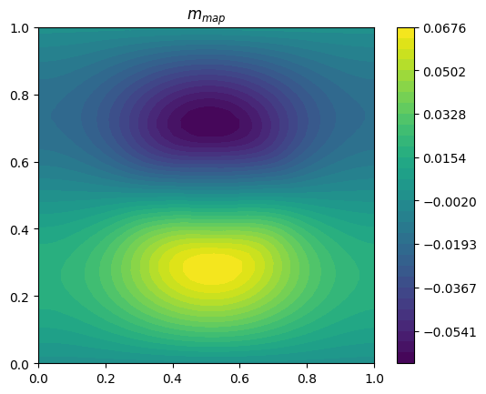
Next we solve the optimization problem. The considered problem seeks to infer the transport in the advection-diffusion equation, in terms of a stream function. Initially the tracer is concentrated on the left, and the observation taken a time \(T\) later has the tracer moved to the right. The variable m_0, which will define our initial guess for the optimization, is set so that the velocity at the center has approximately the correct magnitude for this transport.
As usual we need to define an appropriate inner product associated with derivatives. Here the prior defines a natural inner product – specifically we can use the prior covariance, \(B\), to define an inner product for the dual space \(V^*\).
[4]:
optimizer = TAOSolver(lambda m: forward(m)[2], space, H_0_action=B_action,
                      solver_parameters={"tao_type": "lmvm",
                                         "tao_gatol": 1.0e-5,
                                         "tao_grtol": 0.0,
                                         "tao_gttol": 0.0,
                                         "tao_monitor": None})

m_map = Function(space, name="m_map").assign(m_0)
optimizer.solve(m_map)

reset_manager()
start_manager()
J_mismatch, _, J, u_map = forward(m_map)
stop_manager()
  Iteration information for _tlm_adjoint__Tao_0xc4000003_0_ solve.
  0 TAO,  Function value: 142.531,  Residual: 252.076
  1 TAO,  Function value: 75.6093,  Residual: 78.5923
  2 TAO,  Function value: 68.3955,  Residual: 48.098
  3 TAO,  Function value: 64.8572,  Residual: 33.5383
  4 TAO,  Function value: 60.3369,  Residual: 27.2206
  5 TAO,  Function value: 58.3236,  Residual: 25.1547
  6 TAO,  Function value: 56.863,  Residual: 15.66
  7 TAO,  Function value: 56.2613,  Residual: 23.2133
  8 TAO,  Function value: 56.0512,  Residual: 29.4124
  9 TAO,  Function value: 55.5922,  Residual: 25.9102
 10 TAO,  Function value: 54.986,  Residual: 29.7655
 11 TAO,  Function value: 54.6658,  Residual: 27.5321
 12 TAO,  Function value: 54.0866,  Residual: 31.1733
 13 TAO,  Function value: 53.6629,  Residual: 27.9583
 14 TAO,  Function value: 53.4698,  Residual: 24.8065
 15 TAO,  Function value: 53.1749,  Residual: 22.2047
 16 TAO,  Function value: 53.0568,  Residual: 22.6377
 17 TAO,  Function value: 52.6485,  Residual: 17.693
 18 TAO,  Function value: 52.3048,  Residual: 20.5252
 19 TAO,  Function value: 51.9384,  Residual: 18.2042
 20 TAO,  Function value: 51.6112,  Residual: 12.7694
 21 TAO,  Function value: 51.2598,  Residual: 16.009
 22 TAO,  Function value: 50.8641,  Residual: 13.3265
 23 TAO,  Function value: 50.6379,  Residual: 13.2171
 24 TAO,  Function value: 50.4164,  Residual: 15.321
 25 TAO,  Function value: 49.9947,  Residual: 10.4495
 26 TAO,  Function value: 49.7759,  Residual: 9.19296
 27 TAO,  Function value: 49.6278,  Residual: 13.802
 28 TAO,  Function value: 49.5019,  Residual: 10.8119
 29 TAO,  Function value: 49.4283,  Residual: 11.1461
 30 TAO,  Function value: 49.3206,  Residual: 11.6553
 31 TAO,  Function value: 49.2344,  Residual: 13.5738
 32 TAO,  Function value: 49.0752,  Residual: 12.4629
 33 TAO,  Function value: 48.9742,  Residual: 12.9785
 34 TAO,  Function value: 48.8608,  Residual: 9.69846
 35 TAO,  Function value: 48.7065,  Residual: 12.143
 36 TAO,  Function value: 48.653,  Residual: 11.1146
 37 TAO,  Function value: 48.5809,  Residual: 14.2326
 38 TAO,  Function value: 48.5129,  Residual: 13.3145
 39 TAO,  Function value: 48.4525,  Residual: 13.0799
 40 TAO,  Function value: 48.3492,  Residual: 8.95482
 41 TAO,  Function value: 48.3188,  Residual: 10.6709
 42 TAO,  Function value: 48.2868,  Residual: 9.38934
 43 TAO,  Function value: 48.2554,  Residual: 8.40332
 44 TAO,  Function value: 48.2185,  Residual: 8.02572
 45 TAO,  Function value: 48.1992,  Residual: 7.70232
 46 TAO,  Function value: 48.1456,  Residual: 5.1021
 47 TAO,  Function value: 48.1372,  Residual: 5.88148
 48 TAO,  Function value: 48.1283,  Residual: 5.77235
 49 TAO,  Function value: 48.1185,  Residual: 6.27168
 50 TAO,  Function value: 48.1009,  Residual: 7.03941
 51 TAO,  Function value: 48.0807,  Residual: 6.32074
 52 TAO,  Function value: 48.0587,  Residual: 5.77033
 53 TAO,  Function value: 48.0507,  Residual: 5.9735
 54 TAO,  Function value: 48.0441,  Residual: 6.11227
 55 TAO,  Function value: 48.0354,  Residual: 5.9437
 56 TAO,  Function value: 48.0288,  Residual: 5.77922
 57 TAO,  Function value: 48.0038,  Residual: 4.15742
 58 TAO,  Function value: 47.9882,  Residual: 5.2115
 59 TAO,  Function value: 47.9825,  Residual: 5.35641
 60 TAO,  Function value: 47.9765,  Residual: 5.38986
 61 TAO,  Function value: 47.9743,  Residual: 5.33913
 62 TAO,  Function value: 47.969,  Residual: 5.18917
 63 TAO,  Function value: 47.943,  Residual: 1.76783
 64 TAO,  Function value: 47.9422,  Residual: 1.92053
 65 TAO,  Function value: 47.9411,  Residual: 2.04986
 66 TAO,  Function value: 47.9398,  Residual: 1.97927
 67 TAO,  Function value: 47.9388,  Residual: 1.80429
 68 TAO,  Function value: 47.9366,  Residual: 1.57006
 69 TAO,  Function value: 47.9339,  Residual: 0.475357
 70 TAO,  Function value: 47.9335,  Residual: 0.33338
 71 TAO,  Function value: 47.9327,  Residual: 0.651869
 72 TAO,  Function value: 47.932,  Residual: 0.578996
 73 TAO,  Function value: 47.9312,  Residual: 0.507469
 74 TAO,  Function value: 47.9306,  Residual: 0.39863
 75 TAO,  Function value: 47.9302,  Residual: 0.319103
 76 TAO,  Function value: 47.93,  Residual: 0.313146
 77 TAO,  Function value: 47.9296,  Residual: 0.254428
 78 TAO,  Function value: 47.9294,  Residual: 0.251318
 79 TAO,  Function value: 47.9293,  Residual: 0.245813
 80 TAO,  Function value: 47.9292,  Residual: 0.21433
 81 TAO,  Function value: 47.929,  Residual: 0.220371
 82 TAO,  Function value: 47.9289,  Residual: 0.177634
 83 TAO,  Function value: 47.9288,  Residual: 0.174963
 84 TAO,  Function value: 47.9287,  Residual: 0.178319
 85 TAO,  Function value: 47.9286,  Residual: 0.191331
 86 TAO,  Function value: 47.9286,  Residual: 0.182096
 87 TAO,  Function value: 47.9285,  Residual: 0.163242
 88 TAO,  Function value: 47.9284,  Residual: 0.148827
 89 TAO,  Function value: 47.9283,  Residual: 0.174567
 90 TAO,  Function value: 47.9282,  Residual: 0.147905
 91 TAO,  Function value: 47.9282,  Residual: 0.132948
 92 TAO,  Function value: 47.9281,  Residual: 0.147412
 93 TAO,  Function value: 47.9281,  Residual: 0.153246
 94 TAO,  Function value: 47.928,  Residual: 0.142848
 95 TAO,  Function value: 47.928,  Residual: 0.122535
 96 TAO,  Function value: 47.9279,  Residual: 0.0834194
 97 TAO,  Function value: 47.9279,  Residual: 0.107939
 98 TAO,  Function value: 47.9279,  Residual: 0.0762585
 99 TAO,  Function value: 47.9278,  Residual: 0.0819795
100 TAO,  Function value: 47.9278,  Residual: 0.0840937
101 TAO,  Function value: 47.9278,  Residual: 0.0689404
102 TAO,  Function value: 47.9278,  Residual: 0.0541431
103 TAO,  Function value: 47.9278,  Residual: 0.0663468
104 TAO,  Function value: 47.9278,  Residual: 0.0484867
105 TAO,  Function value: 47.9278,  Residual: 0.045401
106 TAO,  Function value: 47.9278,  Residual: 0.0331168
107 TAO,  Function value: 47.9278,  Residual: 0.0414855
108 TAO,  Function value: 47.9278,  Residual: 0.0321411
109 TAO,  Function value: 47.9278,  Residual: 0.0333852
110 TAO,  Function value: 47.9278,  Residual: 0.0253775
111 TAO,  Function value: 47.9278,  Residual: 0.0276427
112 TAO,  Function value: 47.9278,  Residual: 0.0246038
113 TAO,  Function value: 47.9278,  Residual: 0.0212976
114 TAO,  Function value: 47.9278,  Residual: 0.0176099
115 TAO,  Function value: 47.9278,  Residual: 0.0234908
116 TAO,  Function value: 47.9277,  Residual: 0.0195269
117 TAO,  Function value: 47.9277,  Residual: 0.0195515
118 TAO,  Function value: 47.9277,  Residual: 0.0147668
119 TAO,  Function value: 47.9277,  Residual: 0.0140406
120 TAO,  Function value: 47.9277,  Residual: 0.0196471
121 TAO,  Function value: 47.9277,  Residual: 0.0141066
122 TAO,  Function value: 47.9277,  Residual: 0.0152511
123 TAO,  Function value: 47.9277,  Residual: 0.0134685
124 TAO,  Function value: 47.9277,  Residual: 0.0123951
125 TAO,  Function value: 47.9277,  Residual: 0.0122123
126 TAO,  Function value: 47.9277,  Residual: 0.0094902
127 TAO,  Function value: 47.9277,  Residual: 0.00801
128 TAO,  Function value: 47.9277,  Residual: 0.00915635
129 TAO,  Function value: 47.9277,  Residual: 0.010036
130 TAO,  Function value: 47.9277,  Residual: 0.00843599
131 TAO,  Function value: 47.9277,  Residual: 0.00597544
132 TAO,  Function value: 47.9277,  Residual: 0.00627831
133 TAO,  Function value: 47.9277,  Residual: 0.00565721
134 TAO,  Function value: 47.9277,  Residual: 0.00453639
135 TAO,  Function value: 47.9277,  Residual: 0.00475772
136 TAO,  Function value: 47.9277,  Residual: 0.0042917
137 TAO,  Function value: 47.9277,  Residual: 0.00380307
138 TAO,  Function value: 47.9277,  Residual: 0.00379156
139 TAO,  Function value: 47.9277,  Residual: 0.00279111
140 TAO,  Function value: 47.9277,  Residual: 0.00249391
141 TAO,  Function value: 47.9277,  Residual: 0.00259602
142 TAO,  Function value: 47.9277,  Residual: 0.00220737
143 TAO,  Function value: 47.9277,  Residual: 0.00267611
144 TAO,  Function value: 47.9277,  Residual: 0.00177509
145 TAO,  Function value: 47.9277,  Residual: 0.00171059
146 TAO,  Function value: 47.9277,  Residual: 0.0017233
147 TAO,  Function value: 47.9277,  Residual: 0.00151372
148 TAO,  Function value: 47.9277,  Residual: 0.00138971
149 TAO,  Function value: 47.9277,  Residual: 0.001482
150 TAO,  Function value: 47.9277,  Residual: 0.00117255
151 TAO,  Function value: 47.9277,  Residual: 0.00145642
152 TAO,  Function value: 47.9277,  Residual: 0.00110994
153 TAO,  Function value: 47.9277,  Residual: 0.000840458
154 TAO,  Function value: 47.9277,  Residual: 0.000998263
155 TAO,  Function value: 47.9277,  Residual: 0.000825243
156 TAO,  Function value: 47.9277,  Residual: 0.000684567
157 TAO,  Function value: 47.9277,  Residual: 0.0007538
158 TAO,  Function value: 47.9277,  Residual: 0.000828911
159 TAO,  Function value: 47.9277,  Residual: 0.000572778
160 TAO,  Function value: 47.9277,  Residual: 0.000585657
161 TAO,  Function value: 47.9277,  Residual: 0.000589801
162 TAO,  Function value: 47.9277,  Residual: 0.000538613
163 TAO,  Function value: 47.9277,  Residual: 0.000491709
164 TAO,  Function value: 47.9277,  Residual: 0.000529918
165 TAO,  Function value: 47.9277,  Residual: 0.000453533
166 TAO,  Function value: 47.9277,  Residual: 0.000519699
167 TAO,  Function value: 47.9277,  Residual: 0.000291751
168 TAO,  Function value: 47.9277,  Residual: 0.000361911
169 TAO,  Function value: 47.9277,  Residual: 0.000325335
170 TAO,  Function value: 47.9277,  Residual: 0.000232697
171 TAO,  Function value: 47.9277,  Residual: 0.000317886
172 TAO,  Function value: 47.9277,  Residual: 0.000249638
173 TAO,  Function value: 47.9277,  Residual: 0.000214059
174 TAO,  Function value: 47.9277,  Residual: 0.000248203
175 TAO,  Function value: 47.9277,  Residual: 0.000141242
176 TAO,  Function value: 47.9277,  Residual: 0.000168058
177 TAO,  Function value: 47.9277,  Residual: 0.000171106
178 TAO,  Function value: 47.9277,  Residual: 0.000134217
179 TAO,  Function value: 47.9277,  Residual: 0.000138645
180 TAO,  Function value: 47.9277,  Residual: 0.000153022
181 TAO,  Function value: 47.9277,  Residual: 0.000107386
182 TAO,  Function value: 47.9277,  Residual: 0.000102133
183 TAO,  Function value: 47.9277,  Residual: 8.35358e-05
184 TAO,  Function value: 47.9277,  Residual: 8.80215e-05
185 TAO,  Function value: 47.9277,  Residual: 0.000106023
186 TAO,  Function value: 47.9277,  Residual: 7.38508e-05
187 TAO,  Function value: 47.9277,  Residual: 6.72666e-05
188 TAO,  Function value: 47.9277,  Residual: 5.57236e-05
189 TAO,  Function value: 47.9277,  Residual: 6.79148e-05
190 TAO,  Function value: 47.9277,  Residual: 5.54815e-05
191 TAO,  Function value: 47.9277,  Residual: 4.55044e-05
192 TAO,  Function value: 47.9277,  Residual: 5.13068e-05
193 TAO,  Function value: 47.9277,  Residual: 4.66711e-05
194 TAO,  Function value: 47.9277,  Residual: 4.95998e-05
195 TAO,  Function value: 47.9277,  Residual: 3.7866e-05
196 TAO,  Function value: 47.9277,  Residual: 3.65109e-05
197 TAO,  Function value: 47.9277,  Residual: 3.82517e-05
198 TAO,  Function value: 47.9277,  Residual: 3.5131e-05
199 TAO,  Function value: 47.9277,  Residual: 3.20019e-05
200 TAO,  Function value: 47.9277,  Residual: 3.44756e-05
201 TAO,  Function value: 47.9277,  Residual: 2.70557e-05
202 TAO,  Function value: 47.9277,  Residual: 3.03911e-05
203 TAO,  Function value: 47.9277,  Residual: 2.71093e-05
204 TAO,  Function value: 47.9277,  Residual: 2.05683e-05
205 TAO,  Function value: 47.9277,  Residual: 1.97085e-05
206 TAO,  Function value: 47.9277,  Residual: 1.99219e-05
207 TAO,  Function value: 47.9277,  Residual: 1.8137e-05
208 TAO,  Function value: 47.9277,  Residual: 1.77297e-05
209 TAO,  Function value: 47.9277,  Residual: 1.48771e-05
210 TAO,  Function value: 47.9277,  Residual: 1.77043e-05
211 TAO,  Function value: 47.9277,  Residual: 1.34647e-05
212 TAO,  Function value: 47.9277,  Residual: 1.41654e-05
213 TAO,  Function value: 47.9277,  Residual: 9.37271e-06
[4]:
(True, True)
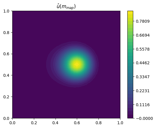
Let’s plot the result.
[5]:
reset_manager()
start_manager()
J_mismatch, _, J, u_map = forward(m_map)
stop_manager()

plot_output(m_map, r"$m_{map}$")
plot_output(u_map, r"$\hat{u} ( m_{map} )$")
Computing uncertainty estimates: Low rank update approximation
We next seek to use Hessian information to quantify the uncertainty in the result of the inference. We use a low-rank update approximation using the methodology of Isaac et al 2015, doi: 10.1016/j.jcp.2015.04.047.
In this approach we consider the mismatch Hessian, \(H_{mismatch}\), obtained by differentiating
twice with respect to the control \(m\). i.e.
We seek eigenpairs \(\lambda_k \in \mathbb{R}\), \(v_k \in V\) such that
where the eigenvectors are \(B^{-1}\)-orthonormal
This leads directly to an expression for a low-rank update approximation for the Hessian inverse, expressed as a low rank update to the prior covariance (equation (20) of Isaac et al 2015, doi: 10.1016/j.jcp.2015.04.047),
which we use to approximate the posterior covariance.
We first perform a higher order Taylor verification using the mismatch Hessian.
[6]:
H_mismatch = CachedHessian(J_mismatch)

dm = Function(space, name="dm").interpolate(
    exp(-((X[0] - 0.3) ** 2 + (X[1] - 0.3) ** 2) / (2 * 0.08 * 0.08)))
min_order = taylor_test(lambda m: forward(m)[0], m_map, J_val=J_mismatch.value, ddJ=H_mismatch, dM=dm, seed=1.0e-4)
assert min_order > 2.99
Error norms, no adjoint   = [0.00379075 0.00214381 0.00113403 0.00058255 0.00029516]
Orders,      no adjoint   = [0.82230944 0.91871228 0.96100471 0.98088892]
Error norms, with adjoint = [4.71842950e-07 5.92286109e-08 7.41905819e-09 9.28147120e-10
 1.15956090e-10]
Orders,      with adjoint = [2.99394059 2.99698629 2.99881065 3.00077491]
We now use SLEPc, seeking the 20 eigenpairs whose eigenvalues have largest magnitude.
Note: There is a notational clash here! Conventially the prior inverse covariance is denoted \(B^{-1}\), but here we use this on the right-hand-side of a generalized eigenproblem, where the associated matrix is also conventially notated \(B\). Here the B_action argument to the HessianEigensolver constructor is set equal to B_inv_action in the call, and the B_inv_action argument is set equal to B_action!
[7]:
esolver = HessianEigensolver(
    H_mismatch, m_map, B_action=B_inv_action, B_inv_action=B_action,
    solver_parameters={"eps_type": "krylovschur",
                       "eps_gen_hermitian": None,
                       "eps_largest_magnitude": None,
                       "eps_nev": 20,
                       "eps_conv_rel": None,
                       "eps_tol": 1.0e-14,
                       "eps_purify": False,
                       "eps_monitor": None})
esolver.solve()
  Eigenvalue approximations and residual norms for _tlm_adjoint__EPS_0xc4000007_0_ solve.
  1 EPS nconv=10 first unconverged value (error) 208.222 (1.53942626e-13)
  2 EPS nconv=16 first unconverged value (error) 118.459 (3.82528711e-14)
  3 EPS nconv=20 first unconverged value (error) 87.915 (2.00950343e-14)
Let’s plot the eigenvalues.
[8]:
lam = esolver.eigenvalues()
assert (lam > 0.0).all()
plt.semilogy(range(1, len(esolver) + 1), lam, "k-")
plt.xlim(0, len(esolver))
plt.xlabel("Eigenvalue index")
plt.ylabel("Eigenvalue")
[8]:
Text(0, 0.5, 'Eigenvalue')
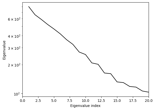
Each eigenvalue indicates some information, added by the observation, over the prior. Specifically each eigenvector \(v_k \in V\) has an associated dual space element defined by the prior inverse covariance, \(q_{v_k} = B^{-1} ( v_k, \cdot ) \in V^*\). If we have an observation for a quantitity of interest defined by a linear functional equal to a (non-zero) multiple of this associated dual space element, and if the posterior were Gaussian, then the associated variance decreases by a factor of one plus the eigenvalue when we add the observation. That is, under the Gaussian approximation, we have
where \(\sigma^2_{q_{v_k},posterior}\) and \(\sigma^2_{q_{v_k},prior}\) are respectively the posterior and prior variance associated with \(q_{v_k}\), and where \(\lambda_k\) is the associated eigenvalue.
Having retained only \(20\) eigenpairs, the smallest eigenvalue obtained is quite a bit bigger than one. This means we might expect to be missing quite a bit of information available in the Hessian if we use a low rank update approximation using only these \(20\) eigenpairs. We’ll return to this issue later.
The linear functional associated with computing the average \(x\)-component of the velocity for \(0.4 < y < 0.6\), \(q_u \in V^*\), satisfies
where \(\mathcal{I}\) is one where \(0.4 < y < 0.6\) and zero elsewhere. We can use this to evaluate an estimate for the posterior mean of this quantity,
[9]:
I = Function(FunctionSpace(mesh, "Discontinuous Lagrange", 0)).interpolate(
    conditional(X[1] > 0.4, 1.0, 0.0) * conditional(X[1] < 0.6, 1.0, 0.0))
q_u = assemble(-(1 / Constant(assemble(I * dx))) * I * test.dx(1) * dx)
print(f"{assemble(q_u(m_map))=}")
assemble(q_u(m_map))=0.26603362165200495
The associated posterior uncertainty estimate is then
[10]:
sigma_u = sqrt(assemble(q_u(esolver.spectral_approximation_solve(q_u))))
print(f"{sigma_u=}")
sigma_u=0.049826943093325984
We can compare this with the prior uncertainty,
[11]:
sigma_prior_q_u = sqrt(assemble(q_u(B_action(q_u))))
print(f"{sigma_prior_q_u=}")
sigma_prior_q_u=0.06809389996419146
i.e. we estimate that the observation has reduced the uncertainty in our estimate for \(q_u( m )\) by about 25%.
Computing uncertainty estimates: Full Hessian inverse
We have made a number of assumptions in order to define the inference problem, but given the problem we have used only two approximations in the uncertainty estimate itself: the local Gaussian assumption (making use of the Hessian), and the low rank update approximation for the Hessian inverse. We now remove the second of these approximations using a Krylov solver, using PETSc. Since we already have an approximation for the Hessian inverse, we can use this to construct a preconditioner in the calculation of a Hessian inverse action.
[12]:
H = CachedHessian(J)

ksp = HessianLinearSolver(H, m_map, solver_parameters={"ksp_type": "cg",
                                                       "ksp_atol": 0.0,
                                                       "ksp_rtol": 1.0e-7,
                                                       "ksp_monitor": None},
                          pc_fn=esolver.spectral_pc_fn())
H_inv_q_u = Function(space, name="H_inv_q_u")
ksp.solve(H_inv_q_u, q_u)
  Residual norms for _tlm_adjoint__KSP_0xc4000009_0_ solve.
  0 KSP Residual norm 9.901063940612e-03
  1 KSP Residual norm 3.846887396923e-03
  2 KSP Residual norm 2.959402172924e-03
  3 KSP Residual norm 1.718696050315e-03
  4 KSP Residual norm 1.325055699763e-03
  5 KSP Residual norm 1.122277413445e-03
  6 KSP Residual norm 9.690002941905e-04
  7 KSP Residual norm 8.439140190241e-04
  8 KSP Residual norm 3.525862866587e-04
  9 KSP Residual norm 5.477244753569e-04
 10 KSP Residual norm 3.121835833383e-04
 11 KSP Residual norm 3.134450820882e-04
 12 KSP Residual norm 2.941740579930e-04
 13 KSP Residual norm 1.381997473824e-04
 14 KSP Residual norm 2.289384303399e-04
 15 KSP Residual norm 1.076096378952e-04
 16 KSP Residual norm 5.271734235858e-05
 17 KSP Residual norm 5.616047775553e-05
 18 KSP Residual norm 5.265159239080e-05
 19 KSP Residual norm 2.521783658860e-05
 20 KSP Residual norm 1.637758855716e-05
 21 KSP Residual norm 3.058528737786e-05
 22 KSP Residual norm 1.532049998254e-05
 23 KSP Residual norm 7.979585813705e-06
 24 KSP Residual norm 1.027004717719e-05
 25 KSP Residual norm 5.229044836309e-06
 26 KSP Residual norm 6.839842962128e-06
 27 KSP Residual norm 4.015886996091e-06
 28 KSP Residual norm 4.402673928099e-06
 29 KSP Residual norm 3.292276914745e-06
 30 KSP Residual norm 2.419410043024e-06
 31 KSP Residual norm 9.394867583164e-07
 32 KSP Residual norm 1.217609278977e-06
 33 KSP Residual norm 2.039049206921e-06
 34 KSP Residual norm 9.341725889835e-07
 35 KSP Residual norm 2.811449319662e-07
 36 KSP Residual norm 4.402614113737e-07
 37 KSP Residual norm 2.961624710683e-07
 38 KSP Residual norm 1.687143968444e-07
 39 KSP Residual norm 1.890661648698e-07
 40 KSP Residual norm 9.740610911599e-08
 41 KSP Residual norm 8.977497357935e-08
 42 KSP Residual norm 7.347374434350e-08
 43 KSP Residual norm 6.582416229412e-08
 44 KSP Residual norm 5.382757249658e-08
 45 KSP Residual norm 6.341360847130e-08
 46 KSP Residual norm 3.470665801808e-08
 47 KSP Residual norm 3.227599902138e-08
 48 KSP Residual norm 1.958410568715e-08
 49 KSP Residual norm 2.301198958079e-08
 50 KSP Residual norm 1.846709667676e-08
 51 KSP Residual norm 1.827263291620e-08
 52 KSP Residual norm 1.189008861456e-08
 53 KSP Residual norm 1.077867596364e-08
 54 KSP Residual norm 7.471548333104e-09
 55 KSP Residual norm 7.808925136195e-09
 56 KSP Residual norm 7.444404082607e-09
 57 KSP Residual norm 4.851473640139e-09
 58 KSP Residual norm 3.990201734499e-09
 59 KSP Residual norm 3.497153443461e-09
 60 KSP Residual norm 3.159027163400e-09
 61 KSP Residual norm 2.518510686472e-09
 62 KSP Residual norm 1.782610592870e-09
 63 KSP Residual norm 1.313695279622e-09
 64 KSP Residual norm 1.090144383730e-09
 65 KSP Residual norm 6.928084128271e-10
Let’s double check that we solved the linear system.
[13]:
residual = Cofunction(space.dual()).assign(
    H.action(m_map, H_inv_q_u)[2] - q_u)
q_u_norm = abs(q_u.dat.data_ro).max()
residual_norm = abs(residual.dat.data_ro).max()
print(f"{residual_norm / q_u_norm=}")
assert residual_norm / q_u_norm < 1.0e-4
residual_norm / q_u_norm=np.float64(1.608633886866077e-05)
Our new uncertainty estimate, using the full Hessian, is
[14]:
sigma_u = sqrt(assemble(q_u(H_inv_q_u)))
print(f"{sigma_u=}")
sigma_u=0.031200525962623942
This reveals that our partial eigenspectrum estimate did indeed miss quite a bit of relevant information available in the Hessian. In fact with the full Hessian we estimate a reduction in uncertainty of about 55%.