Defining custom operations

This notebook describes the tlm_adjoint ‘escape hatch’ mechanism, which allows custom operations to be defined, recorded by the internal manager, and used in higher order derivative calculations.

The approach used by tlm_adjoint to define custom operations is described in

James R. Maddison, Daniel N. Goldberg, and Benjamin D. Goddard, ‘Automated calculation of higher order partial differential equation constrained derivative information’, SIAM Journal on Scientific Computing, 41(5), pp. C417–C445, 2019, doi: 10.1137/18M1209465

We assume real spaces and a real build of Firedrake throughout.

Forward problem

We consider the Poisson equation in the unit square domain

\[\nabla^2 u = m \quad \text{on} ~ \Omega = \left( 0, 1 \right)^2,\]

with

\[\int_\Omega m = 0,\]

subject to boundary conditions

\[\nabla u \cdot \hat{n} = 0,\]

where \(\hat{n}\) is an outward unit normal on the boundary \(\partial \Omega\) of the domain \(\Omega\).

We consider a continuous Galerkin discretization, now seeking \(u \in V\) such that

\[\forall \zeta \in V \qquad \int_\Omega \nabla \zeta \cdot \nabla u = -\int_\Omega \zeta m,\]

where \(V\) is a real \(P_1\) continuous finite element space defining functions on the domain \(\Omega = \left( 0, 1 \right)^2\). \(m \in V\) is now defined via

\[m = \mathcal{I} \left[ \cos \left( \pi x \right) \cos \left( \pi y \right) \right] - k,\]

where \(\mathcal{I}\) maps to an element of \(V\) through interpolation at mesh vertices, and where \(k\) is defined so that \(\int_\Omega m = 0\).

As stated the discrete problem does not have a unique solution – given any solution \(u_0\) to the problem we can define a new solution \(u_1 = u_0 + c_1\) for any scalar \(c_1\). We need to identify a solution by supplying an appropriate constraint. We will use the constraint

\[\sum_i \tilde{u}_i = 0,\]

where the \(\tilde{u}_i\) are the degrees of freedom associated with \(u \in V\).

An implementation using Firedrake, solving for \(u\) and then computing \(\frac{1}{2} \int_\Omega u^2\), takes the form

[1]:

%matplotlib inline

from firedrake import *
from firedrake.pyplot import tricontourf

import matplotlib.pyplot as plt
import numpy as np

mesh = UnitSquareMesh(10, 10)
X = SpatialCoordinate(mesh)
space = FunctionSpace(mesh, "Lagrange", 1)
test, trial = TestFunction(space), TrialFunction(space)


def forward(m):
    k = Constant(assemble(m * dx) / assemble(Constant(1.0) * dx(mesh)))
    m_tilde = Function(m.function_space(), name="m_tilde").interpolate(m - k)

    u = Function(space, name="u")
    nullspace = VectorSpaceBasis(comm=u.comm, constant=True)

    solve(inner(grad(trial), grad(test)) * dx == -inner(m_tilde, test) * dx,
          u, nullspace=nullspace, transpose_nullspace=nullspace,
          solver_parameters={"ksp_type": "cg", "pc_type": "hypre",
                             "pc_hypre_type": "boomeramg",
                             "ksp_rtol": 1.0e-10, "ksp_atol": 1.0e-16})

    J = assemble(0.5 * inner(u, u) * dx)
    return u, J


m = Function(space, name="m").interpolate(cos(pi * X[0]) * cos(pi * X[1]))

u, J = forward(m)


def plot_output(u, title):
    r = (u.dat.data_ro.min(), u.dat.data_ro.max())
    eps = (r[1] - r[0]) * 1.0e-12
    p = tricontourf(u, np.linspace(r[0] - eps, r[1] + eps, 32))
    plt.gca().set_title(title)
    plt.colorbar(p)
    plt.gca().set_aspect(1.0)


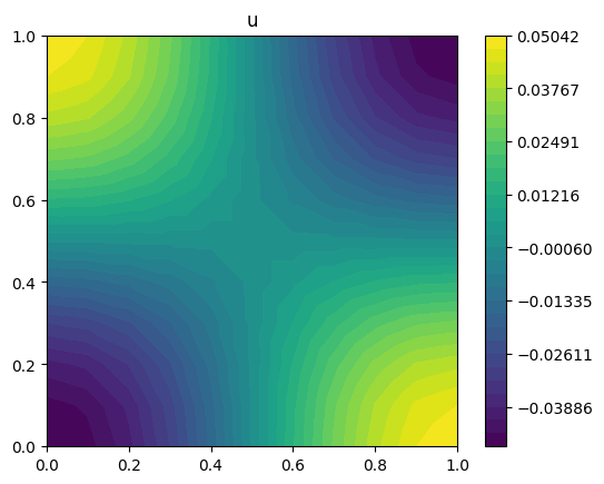
plot_output(u, title="u")

../_images/examples_6_custom_operations_1_0.png

Adding tlm_adjoint

Next we add the use of tlm_adjoint, which requires some minor modification of the forward code.

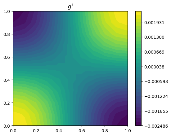
compute_gradient is used to compute the derivative of \(\frac{1}{2} \int_\Omega u^2\) with respect to \(m\), subject to the contraint that the forward problem is solved. The derivative is visualized using a Riesz map defined by the \(L^2\) inner product. A Taylor remainder convergence test is used to verify the derivative.

Note that, given an arbitrary \(m \in V\), we define

\[\tilde{m} = m - \frac{\int_\Omega m}{\int_\Omega 1},\]

so that \(\int_\Omega \tilde{m} = 0\), and use \(\tilde{m}\) in place of \(m\) when solving the discrete Poisson problem.

[2]:

%matplotlib inline

from firedrake import *
from tlm_adjoint.firedrake import *
from firedrake.pyplot import tricontourf

import matplotlib.pyplot as plt
import numpy as np

np.random.seed(54151610)
reset_manager()

mesh = UnitSquareMesh(10, 10)
X = SpatialCoordinate(mesh)
space = FunctionSpace(mesh, "Lagrange", 1)
test, trial = TestFunction(space), TrialFunction(space)


def forward(m):
    v = Constant(name="v")
    Assembly(v, Constant(1.0) * dx(mesh)).solve()
    k = Constant(name="k")
    Assembly(k, (m / v) * dx).solve()
    m_tilde = Function(m.function_space(), name="m_tilde").interpolate(m - k)

    u = Function(space, name="u")
    nullspace = VectorSpaceBasis(comm=u.comm, constant=True)

    solve(inner(grad(trial), grad(test)) * dx == -inner(m_tilde, test) * dx,
          u, nullspace=nullspace, transpose_nullspace=nullspace,
          solver_parameters={"ksp_type": "cg", "pc_type": "hypre",
                             "pc_hypre_type": "boomeramg",
                             "ksp_rtol": 1.0e-10, "ksp_atol": 1.0e-16})

    J = Functional(name="J")
    J.assign(0.5 * inner(u, u) * dx)
    return u, J


m = Function(space, name="m").interpolate(cos(pi * X[0]) * cos(pi * X[1]))

start_manager()
u, J = forward(m)
stop_manager()

dJ = compute_gradient(J, m)


def plot_output(u, title):
    r = (u.dat.data_ro.min(), u.dat.data_ro.max())
    eps = (r[1] - r[0]) * 1.0e-12
    p = tricontourf(u, np.linspace(r[0] - eps, r[1] + eps, 32))
    plt.gca().set_title(title)
    plt.colorbar(p)
    plt.gca().set_aspect(1.0)


plot_output(u, title="u")
plot_output(dJ.riesz_representation("L2"), title=r"$g^\sharp$")


def forward_J(m):
    _, J = forward(m)
    return J


min_order = taylor_test(forward_J, m, J_val=J.value, dJ=dJ)
assert min_order > 1.99

Error norms, no adjoint   = [6.16667546e-08 3.06309860e-08 1.52648952e-08 7.61979814e-09
 3.80673670e-09]

Orders,      no adjoint   = [1.00950111 1.00477412 1.002393   1.00119799]

Error norms, with adjoint = [8.09565105e-10 2.02391272e-10 5.05978163e-11 1.26494529e-11
 3.16236247e-12]

Orders,      with adjoint = [2.00000003 2.00000005 2.00000013 2.00000034]

../_images/examples_6_custom_operations_3_4.png

../_images/examples_6_custom_operations_3_5.png

Defining a custom `Equation`

Since the \(u\) we have computed should satisfy

\[\sum_i \tilde{u}_i = 0,\]

we should have that the derivative of this quantity with respect to \(m\), subject to the forward problem being solved, is zero. We will compute this derivative by defining a custom operation which sums the degrees of freedom of a finite element discretized function. We can do this by inheriting from the Equation class and implementing appropriate methods.

[3]:

from tlm_adjoint import Equation


class Sum(Equation):
    def __init__(self, x, y):
        super().__init__(x, deps=(x, y), nl_deps=(), ic=False, adj_ic=False,
                         adj_type="conjugate_dual")

    def forward_solve(self, x, deps=None):
        if deps is None:
            deps = self.dependencies()
        _, y = deps
        with y.dat.vec_ro as y_v:
            y_sum = y_v.sum()
        x.assign(y_sum)

    def adjoint_jacobian_solve(self, adj_x, nl_deps, b):
       return b

    def adjoint_derivative_action(self, nl_deps, dep_index, adj_x):
        if dep_index != 1:
            raise ValueError("Unexpected dep_index")

        _, y = self.dependencies()
        b = Cofunction(var_space(y).dual())
        adj_x = float(adj_x)
        b.dat.data[:] = -adj_x
        return b

    def tangent_linear(self, tlm_map):
        tau_x, tau_y = (tlm_map[dep] for dep in self.dependencies())
        if tau_y is None:
            return ZeroAssignment(tau_x)
        else:
            return Sum(tau_x, tau_y)

We’ll investgate how this is put together shortly.

First, we check that the Sum class works. In the following we check that we can compute the sum of the degrees of freedom of a function, and then use Taylor remainder convergence tests to verify a first order tangent-linear calculation, a first order adjoint calculation, and a reverse-over-forward adjoint calculation of a Hessian action.

[4]:

from firedrake import *
from tlm_adjoint.firedrake import *

import numpy as np

np.random.seed(13561700)
reset_manager()


def forward(m):
    m_sum = Float(name="m_sum")
    Sum(m_sum, m).solve()

    J = m_sum ** 3

    return m_sum, J


def forward_J(m):
    _, J = forward(m)
    return J


mesh = UnitIntervalMesh(10)
x, = SpatialCoordinate(mesh)
space = FunctionSpace(mesh, "Discontinuous Lagrange", 0)

m = Function(space, name="m")
m.interpolate(exp(-x) * sin(pi * x))
with m.dat.vec_ro as m_v:
    m_sum_ref = m_v.sum()

start_manager()
m_sum, J = forward(m)
stop_manager()

# Verify the forward calculation

print(f"{float(m_sum)=}")
print(f"{m_sum_ref=}")
assert abs(float(m_sum) - m_sum_ref) == 0.0

# Verify tangent-linear and adjoint calculations

min_order = taylor_test_tlm(forward_J, m, tlm_order=1)
assert min_order > 1.99

min_order = taylor_test_tlm_adjoint(forward_J, m, adjoint_order=1)
assert min_order > 1.99

min_order = taylor_test_tlm_adjoint(forward_J, m, adjoint_order=2)
assert min_order > 1.99

float(m_sum)=3.97146153200585
m_sum_ref=3.97146153200585
Error norms, no tangent-linear   = [1.4597981  0.72709661 0.36284904 0.18124987 0.09058129]

Orders,      no tangent-linear   = [1.00554988 1.00277762 1.00138948 1.00069491]

Error norms, with tangent-linear = [1.11954288e-02 2.79527053e-03 6.98369299e-04 1.74536283e-04
 4.36270656e-05]

Orders,      with tangent-linear = [2.00184997 2.00092587 2.00046316 2.00023164]

Error norms, no adjoint   = [1.68516173 0.83885294 0.41849655 0.20901605 0.10445   ]

Orders,      no adjoint   = [1.00639725 1.00320219 1.00160198 1.00080121]

Error norms, with adjoint = [1.48897315e-02 3.71693487e-03 9.28546465e-04 2.32050710e-04
 5.80019391e-05]

Orders,      with adjoint = [2.00213243 2.0010674  2.00053399 2.00026707]

Error norms, no adjoint   = [3.70748562 1.85093251 0.92476368 0.46220619 0.23105919]

Orders,      no adjoint   = [1.00218881 1.00109565 1.00054814 1.00027415]

Error norms, with adjoint = [1.12412164e-02 2.81030409e-03 7.02576023e-04 1.75644006e-04
 4.39110014e-05]

Orders,      with adjoint = [2. 2. 2. 2.]

We can now use Sum with the Poisson solver. We find, as expected, that the derivative of the sum of the degrees of freedom for \(u\) with respect to \(m\), subject to the forward problem being solved, is zero.

[5]:

%matplotlib inline

from firedrake import *
from tlm_adjoint.firedrake import *

import matplotlib.pyplot as plt
import numpy as np

reset_manager()

mesh = UnitSquareMesh(10, 10)
X = SpatialCoordinate(mesh)
space = FunctionSpace(mesh, "Lagrange", 1)
test, trial = TestFunction(space), TrialFunction(space)


def forward(m):
    v = Constant(name="v")
    Assembly(v, Constant(1.0) * dx(mesh)).solve()
    k = Constant(name="k")
    Assembly(k, (m / v) * dx).solve()
    m_tilde = Function(m.function_space(), name="m_tilde").interpolate(m - k)

    u = Function(space, name="u")
    nullspace = VectorSpaceBasis(comm=u.comm, constant=True)

    solve(inner(grad(trial), grad(test)) * dx == -inner(m_tilde, test) * dx,
          u, nullspace=nullspace, transpose_nullspace=nullspace,
          solver_parameters={"ksp_type": "cg", "pc_type": "hypre",
                             "pc_hypre_type": "boomeramg",
                             "ksp_rtol": 1.0e-10, "ksp_atol": 1.0e-16})

    J = Functional(name="J")
    J.assign(0.5 * inner(u, u) * dx)

    u_sum = Constant(name="u_sum")
    Sum(u_sum, u).solve()

    K = Functional(name="K")
    K.assign(u_sum)

    return u, J, K


m = Function(space, name="m").interpolate(cos(pi * X[0]) * cos(pi * X[1]))

start_manager()
u, J, K = forward(m)
stop_manager()

dJ, dK = compute_gradient((J, K), m)

dK_norm = abs(dK.dat.data_ro).max()
print(f"{dK_norm=}")

assert dK_norm == 0.0

dK_norm=0.0

`Equation` methods

We now return to the definition of the Sum class, and consider each method in turn.

`init`

def __init__(self, x, y):
    super().__init__(x, deps=(x, y), nl_deps=(), ic=False, adj_ic=False,
                     adj_type="conjugate_dual")

The arguments passed to the base class constructor are:

The output of the forward operation, x.
deps: Defines all inputs and outputs of the forward operation.
nl_deps: Defines elements of deps on which the associated adjoint calculations can depend.
ic: Whether the forward operation accepts a non-zero ‘initial guess’.
adj_ic: Whether an adjoint solve accepts a non-zero ‘initial guess’.
adj_type: Either "primal" or "conjugate_dual" defining the space for an associated adjoint variable.

For this operation there is one output x and one input y. The operation is defined by the forward residual function

\[F \left( x, y \right) = x - \sum_i \tilde{u}_i.\]

Given a value for \(y\) the output of the operation is defined to be the \(x\) for which \(F \left( x, y \right) = 0\). \(F\) depends linearly on both \(x\) and \(y\), and so associated adjoint calculations are independent of both \(x\) and \(y\). Hence we set deps=(x, y) and nl_deps=().

ic and adj_ic are used to indicate whether non-zero initial guesses should be supplied to forward and adjoint iterative solvers respectively. Here we do not use iterative solvers, and so no non-zero initial guesses are needed. Hence we set ic=False and adj_ic=False.

adj_type indicates whether an adjoint variable associated with the operation is:

In the same space as x. This is the case where \(F\) maps to an element in the antidual space associated with \(x\), and is indicated with adj_x_type="primal". A typical example of this case is an operation defined via the solution of a finite element variational problem.
In the antidual space associated with the space for x. This is the case where \(F\) maps to an element in same space as \(x\), and is indiciated with adj_x_type="conjugate_dual".

`forward_solve`

def forward_solve(self, x, deps=None):
    if deps is None:
        deps = self.dependencies()
    _, y = deps
    with y.dat.vec_ro as y_v:
        y_sum = y_v.sum()
    x.assign(y_sum)

This method computes the output of the forward operation, storing the result in x. deps is used in rerunning the forward calculation when making use of a checkpointing schedule. If supplied, deps contains values associated with the dependencies as defined in the constructor (defined by the deps argument passed to the base class constructor). Otherwise the values contained in self.dependencies() are used.

`adjoint_jacobian_solve`

def adjoint_jacobian_solve(self, adj_x, nl_deps, b):
   return b

Solves a linear problem

\[\frac{\partial F}{\partial x}^T \lambda = b,\]

for the adjoint solution \(\lambda\), returning the result. The right-hand-side \(b\) is defined by the argument b. In this example \(\partial F / \partial x\) is simply the identity, and so \(\lambda = b\).

adj_x can contain an initial guess for an iterative solver used to compute \(\lambda\). nl_deps contains values associated with the forward dependencies of the adjoint, as defined in the constructor (defined by the nl_deps argument passed to the base class constructor).

`adjoint_derivative_action`

def adjoint_derivative_action(self, nl_deps, dep_index, adj_x):
    if dep_index != 1:
        raise ValueError("Unexpected dep_index")

    _, y = self.dependencies()
    b = Cofunction(var_space(y).dual())
    adj_x = float(adj_x)
    b.dat.data[:] = -adj_x
    return b

Computes

\[\frac{\partial F}{\partial v}^T \lambda,\]

where \(v\) is the dep_indexth dependency (for the dependencies defined by the deps argument passed to the base class constructor). Again nl_deps contains values associated with the forward dependencies of the adjoint, as defined in the constructor.

`tangent_linear`

def tangent_linear(self, tlm_map):
    tau_x, tau_y = (tlm_map[dep] for dep in self.dependencies())
    if tau_y is None:
        return ZeroAssignment(tau_x)
    else:
        return Sum(tau_x, tau_y)

Constructs a tangent-linear operation, for a tangent-linear computing directional derivatives with respect to the control defined by M with direction defined by dM. tlm_map is used to access tangent-linear variables.

The new operation is defined by the residual function

\[F_\tau \left( \tau_x, \tau_y \right) = \frac{\partial F}{\partial x} \tau_x + \frac{\partial F}{\partial y} \tau_y,\]

where \(\tau_x\) and \(\tau_y\) are the tangent-linear variables associated with \(x\) and \(y\) respectively. Given a value for \(\tau_y\) the output of the operation is defined to be the \(\tau_x\) for which \(F_\tau \left( \tau_x, \tau_y \right) = 0\).

Note that this method returns an Equation instance – here either a ZeroAssignment, for the case where the tangent-linear operation sets a tangent-linear variable equal to zero, or another Sum. This new operation can then be recorded by the internal manager, so that reverse-over-forward algorithmic differentiation can be applied.

Reference dropping

An important method, not defined in this example, is the drop_references method. This method is used to drop references to forward data. For example if an Equation subclass defines a Function attribute _function, then the drop_references method might look like

def drop_references(self):
    super().drop_references()
    self._function = var_replacement(self._function)

Here var_replacement returns a ‘symbolic only’ version of self._function, which can for example be used in UFL expressions, but which has no associated value.