Visualizing derivatives

When we differentiate a functional with respect to a finite element discretized function in some discrete function space \(V\), we do not obtain a function in \(V\), but instead obtain an element of the associated dual space \(V^*\). This notebook describes how a Riesz map can be used to construct a function, associated with the derivative, which can be visualized.

This example makes use of tlm_adjoint with the Firedrake backend, and we assume real spaces and a real build of Firedrake throughout.

Forward problem

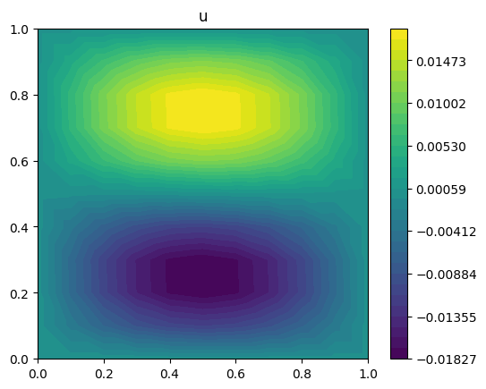
We consider the solution \(u \in V\) of a discretization of the Poisson equation subject to homogeneous Dirichlet boundary conditions,

\[\forall \zeta \in V_0 \qquad \int_\Omega \nabla \zeta \cdot \nabla u = -\int_\Omega \zeta m,\]

where \(V\) is a real \(P_1\) continuous finite element space defining functions on the domain \(\Omega = \left( 0, 1 \right)^2\), with \(m \in V\), and where \(V_0\) consists of the functions in \(V\) which have zero trace. We define a functional

\[J \left( u \right) = \int_\Omega \left( 1 - x \right)^4 u^2,\]

where \(x\) and \(y\) denote Cartesian coordinates in \(\mathbb{R}^2\).

We first solve the forward problem for

\[m = \mathcal{I} \left[ \sin \left( \pi x \right) \sin \left( 2 \pi y \right) \right],\]

where \(\mathcal{I}\) maps to an element of \(V\) through interpolation at mesh vertices.

%matplotlib inline

from firedrake import *
from tlm_adjoint.firedrake import *
from firedrake.pyplot import tricontourf

import matplotlib.pyplot as plt
import numpy as np

mesh = UnitSquareMesh(10, 10)
X = SpatialCoordinate(mesh)
space = FunctionSpace(mesh, "Lagrange", 1)
test, trial = TestFunction(space), TrialFunction(space)
m = Function(space, name="m").interpolate(sin(pi * X[0]) * sin(2 * pi * X[1]))


def forward(m):
    u = Function(space, name="u")
    solve(inner(grad(trial), grad(test)) * dx == -inner(m, test) * dx,
          u, DirichletBC(space, 0.0, "on_boundary"))

    J = Functional(name="J")
    J.assign(((1.0 - X[0]) ** 4) * u * u * dx)
    return u, J


u, J = forward(m)

print(f"{J.value=}")


def plot_output(u, title):
    r = (u.dat.data_ro.min(), u.dat.data_ro.max())
    eps = (r[1] - r[0]) * 1.0e-12
    p = tricontourf(u, np.linspace(r[0] - eps, r[1] + eps, 32))
    plt.gca().set_title(title)
    plt.colorbar(p)
    plt.gca().set_aspect(1.0)


plot_output(u, title="u")

J.value=9.711060188691798e-06

First order adjoint

We can differentiate a functional respect to \(m\) using compute_gradient. Specifically we compute the derivative of \(\hat{J} = J \circ \hat{u}\), where \(\hat{u}\) is the function which maps from the control \(m\) to the solution to the discretized Poisson problem.

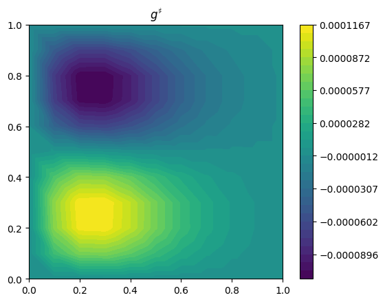
When we compute a derivative of a functional with respect to a finite element discretized function using the adjoint method the result is not a function, but is instead a member of a dual space. Here we have \(m \in V\), and the derivative of \(\hat{J}\) with respect to \(m\) is a member of the associated dual space \(V^*\). In order to visualize this derivative we first need to map it to \(V\). We can do this using a Riesz map. This is not uniquely defined, but here we choose to define a Riesz map using the \(L^2\) inner product.

Being precise the function we visualize, \(g^\sharp \in V\), is defined such that

\[\forall \zeta \in V \qquad \left. \frac{d \hat{J} \left( m + \alpha \zeta \right)}{d \alpha} \right|_{\alpha = 0} = \int_\Omega \zeta g^\sharp,\]

where \(\alpha\) is a scalar.

reset_manager()

start_manager()
u, J = forward(m)
stop_manager()

print(f"{J.value=}")
plot_output(u, title="u")


dJdm = compute_gradient(J, m)
plot_output(dJdm.riesz_representation("L2"), title=r"$g^\sharp$")

J.value=9.711060188691798e-06

Hessian action

Next we seek to differentiate \(\hat{J}\) twice with respect to \(m\). However the second derivative defines a bilinear operator. This can be represented as a matrix – a Hessian matrix – but the number of elements in this matrix is equal to the square of the number of degrees of freedom for \(m\).

Instead of computing the full second derivative we can compute its action on a given direction \(\zeta \in V\). The degrees of freedom associated with the result define the action of the Hessian matrix on a vector – specifically the action of the Hessian matrix on the vector consisting of the degrees of freedom for \(\zeta\).

We do this in two stages. First we compute a directional derivative,

\[\left. \frac{d \hat{J} \left( m + \alpha \zeta \right)}{d \alpha} \right|_{\alpha=0},\]

computed using the tangent-linear method. We consider the case where \(\zeta = 1\).

reset_manager()

zeta = Function(space).interpolate(Constant(1.0))
configure_tlm((m, zeta))

start_manager()
u, J = forward(m)
stop_manager()

print(f"{J.value=}")
plot_output(u, title="u")

dJdm_zeta = var_tlm(J, (m, zeta))
print(f"{dJdm_zeta.value=}")

J.value=9.711060188691798e-06
dJdm_zeta.value=1.158069356484376e-06

Next we compute the derivative of this derivative using the adjoint method.

Again we need to remember that the result is a member of the dual space \(V^*\), and is not a function, so we again use a Riesz map to visualize it. Here we use the same Riesz map as before, defined using the \(L^2\) inner product.

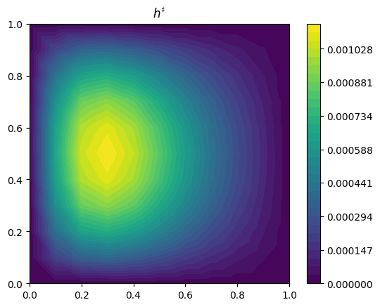
Being precise the function we visualize, \(h^\sharp \in V\), is defined such that

\[\forall \chi \in V \qquad \left. \frac{\partial^2 \hat{J} \left( m + \alpha \zeta + \beta \chi \right)}{\partial \beta \partial \alpha} \right|_{\alpha = 0, \beta = 0} = \int_\Omega \chi h^\sharp,\]

where \(\zeta \in V\) defines the direction on which the action is computed, and \(\alpha\) and \(\beta\) are scalars.

d2Jdm2_zeta = compute_gradient(dJdm_zeta, m)
plot_output(d2Jdm2_zeta.riesz_representation("L2"), title=r"$h^\sharp$")